| |
 Click to Enlarge
|
LEVEL CONTROL LOOP TRAINER MODEL IBL-1
Level Control Process Loop Trainer Model LVL-1 is intended to study the level control dynamics under closed loop control. This equipment finds applications in Instrumentation laboratory and training organizations. Using this trainer one can study the rudiments of level control. The level control loop trainer has all the required hardware and software needed for controlling level in a tank. The instrument consists of a cylindrical water tank of approximately 30cm high water column with 16cm diameter. A centrifugal pump water from a built-in sump, through a control valve and a Rotometer into this tank. The control valve regulates the rate of flow under software command. A Rotometer displays the flow rate. The level of water in the water tank is displayed by a separate 30cm high sight glass tube. A level transmitter produces current in the range of 4mA to 20mA proportional to the height of water column in the water tank. This level transmitter is used as feedback transducer, to communicate the level to the controller in terms of current. The controller (software driven) determines the current water level. The difference in desired level and current water level is computed. Based on this information the controller determines the desired control action. If the current water level is below the desired level, the control valve allows more water to flow into the tank. As the error reduces, the flow of the water reduces, thus achieving a PID control. If the current water level is above the desired level, a solenoid valve automatically opens and allows the excess water present in the water tank to drain. Hence, the desired level is achieved. In order to provide a disturbance, a hand valve is used. On opening this hand valve, the water from the water tank is discharged into the sump directly, resulting in fall in water level in the tank.
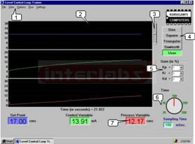
In order to assist in conducting the experiment, several WINDOW based features are provided. They are: This is the process screen. This screen is used to do the following Input Parameters:
1. Set point of desired level in Cms or
Set the variable set point by using function generator inputs as SINE, SQUARE, TRIANGLE, SAW TOOTH.
2. Set the Proportional (kp) gain in the range of 1 to 100%
Set the Integral (ki) gain in the range of 1 to 100%
Set the Differential (kd) gain in the range of 1 to 100%
Sampling time in terms of mS. Output Parameters:These are displayed in response to the above parameters. These are displayed as a function of comparing the feedback parameters.
1. Process variable in Cms
2. Controlling variable that is responsible controlling the process to restore close to the set point.
Graphs: These are stored dynamically, and will be displayed any time. When show graph option is selected, the controlling process stops, and gets ready to display the
trend. There are varieties of statical graphs that can be generated as a consequence of data logging. These graphs can also be printed. How to view the graphs: The following possibilities are available to view the graph. They are:
Show Combined Graph : When this option is selected, all the process parameters appear in a single graph, as shown below. All the three parameters overlap one above the other. In this mode all the three parameters namely (a) setpoint (b) process variable, and (c) Controlling force are all displayed in the same screen. Show Individual Graph: When this option is selected, the process parameters are displayed as individual graphs in the same screen, as shown below. This distinguishes one graph from the other.
Show Combined Graph : : When this option is selected, the whole run is displayed at once, as shown below. When this is selected, the complete trend from the start is displayed.
Zoom: This feature allows the user to zoom into a specific portion of the graph. Move the cursor to the point where you want the zoomed portion to start, as shown below.
Insert markers: A marker will appear as a gray line on the graph. For each marker, indicator labels appear, indicating the values of the corresponding process parameters. By inserting markers, a specific portion of the trend may be observed more closely. This option is necessary as, some times the process takes long time to settle down. At this time, it is a good method to move your cursor to a specific portion of your process and view that zone, which is critical for analysis.
Using this trainer, we can perform the following experiments. 1. Study characteristics of a level transmitter. I.e. relation between water level and the current generated by the level transmitter. Plot a graph LEVEL Vs CURRENT. This information is useful to design lookup table, while designing a controller.
2. Study a program to tabulate a relationship between a digital to analog converter (DAC), and the 4 - 20mA current generated. This current can be monitored on an analog and digital indicators. Tabulate this relation DAC number Vs current output (4 - 20mA). Plot a graph. This information is useful in setting a control function to I - P converter.
3. Study a program to understand the relation between current to pressure conversion. In this program, 4 to 20mA currents are used to activate a current to pressure (I to P) converter. For 4mA current, the I-P converter provides 3 PSI (0.2kg/cm2) at it's output port. For 20mA current the output pressure will be 15PSI (1 Kg/cm2). Plot a graph.
4. Study a program to activate the solenoid. This study demonstrates how to discharge water from the water tank.
5. Study a program to change the stem position of control valve, under software control. The stem of the control valve changes its position from one extreme position to the other (usually 0 to 10-15mm) under air pressure. For 3PSI, the stem is in initial position, i.e., and 0mm. For 15PSI, the stem changes its position to the other end. This up/down movement causes, valve to open and close. This action changes the water flow through the pipeline. The water flow can be changed in the range of 3 to 10 Liters/min (LPM). This demonstrates how to change water flow pattern by software.
Tabulate the input pressure (3-15 PSI) VS stem position (0 - 10mm). Plot a graph
6. Study a program to measure, rate of change in the stem's position from 0% to 100% open and 100% to 0% open. This will be used later to study dynamics of control valve. This program demonstrates how quickly water flow can be changed. Plot a graph
7. Study a program to measure the change in water flow rate by observing Rotometer, for different control valve settings.
The setting can be from 0% to 100% open condition and 100% to 0% open.
Tabulate the flow rate (3 to 10LPM) VS valve position (0 to 100%). Plot a graph.
8. RUN PID CONTROL PROGRAM.
Many more experiments can be conducted in the above equipment, as every input and output element is accessible by software. You can formulate an experimental scheme to suit your syllabi needs.
Specifications: a) Control Valve:
Fluid : Water.
Body form : Globe
Size body/port/Cv : 1/2"- 1/4" - 2.0Gpm.
Body material : A216 Gr.WCB
Trim form / Material : Contoured / SS316.
Flow chart/Direction : Linear
Actuator type : Diaphragm.
Spring Range : 0.2 - 1.0 Kg/cm2.
Valve action : Air to open.
Total stem travel : 14.3mm. b) Hand Operated Valves:
Quantity : 1 nos.
Size :1/2".
Coating : Nickel.
Type : Close open close. c) Level Transmitter:
Probe type : Stillwell rod
Probe size : ?? dia
Probe material : ss304
Probe insulation : Teflon Insulated
Enclosure : Weather proof d) Electro-Pneumatic Converter:
Input : 4-20mA.
Output : 3-15 PSI.
Input Resistance : 90 Ohms.
Characteristics : Linear to input current.
Air Supply : 1.4Kg/cm2.
Consumption : 30 L/Hr typical.
Pressure : 1.4 bar.
Connection : 1/4" NPT.
Mounting : Wall. e) Air Filter Regulator:
Service Media : Air
Indicator : Pr gauges
Max input : 10Kg/cm2.
Hose connection : 1/4" BSP. f) Solenoid:
Service : Water.
Coil voltage : 220 VAC.
Service connection : 1/2". g) Current Meters:
Analog : 25mA FSD ?2 Nos h) Rotometer:
Service : Water.
Connection : 1/2". Range : 0 to 10.5 LPM.
Metering tube : Borosilicate.
Float : SS 304.
Needle : Provided, integral. i) Water Pump:
Voltage : 220V AC.
Lift : 2000 Lt./Hr to 20Meters high.
Service : Water
Connection : 3/4" upstream.
1/2" reduced for downstream. j) Water Tank (sump):
Capacity : 25 Lt. What you must provide the following facilities at your cost, at the time of installation:
You have to provide compressed air @ 5kg/cm2 from your in-house compressor.
Constant water line to be provided by you for filling the water tank and discharge pipelines must be provided to drain the water from the tank after the completion of the experiment.
You must provide an IBM Computer or Compatible system. It must have at least one vacant ISA slot on the motherboard, to enable the ADD-ON card to be inserted, which will communicate with the trainer. The minimum configuration of the system must be any Intel make standard CPU, 32MB RAM, one 1.44?FDD, HDD with any capacity, CD ROM drive, and a color monitor.
You must provide the necessary electrical fittings at 230V AC single phase, and accessories, observing all the safety standard features, like circuit breakers, safety switches and fuses etc, so that the operator will work under safe environment. Proper electrical grounding (earth) must be provided to the instrument setup as a whole.
This requires 10 Sq.ft floor space for conducting experiments by the students or trainee.
Good electrical connection, with proper earthing is required.
Mobility: Mounted on robust caster wheels
Dimensions: 4' X 2' X 6' (L, B,H)
Specifications are subject to change without notice. Changes in specifications may be effected even after receiving confirmed purchase ORDER.
See Enlarge
|
|
|
|
 Click to Enlarge
|
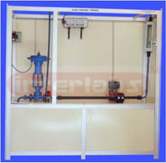
FLOW CONTROL LOOP TRAINER MODEL IBL-1
Flow Control Process Loop Trainer, Model FCL-1 is intended to study, the flow control dynamics in a closed loop instrument. This equipment is used in instrumentation laboratories, process control training organizations, R&D labs. Flow of a liquid in a pipeline is a common phenomenon. Any fluid or for that matter any liquid has to pass in a pipeline only. Control instrument comes into picture, whenever regulated flow is desired.
For Example:
Assumption 1: Crude oil is flowing in a pipeline at the rate of 100 liters/minute. The oil is pumped from an offshore ship, to a refinery located at a distance of 10 Kilometers. Crude arriving at the refinery is discharged into five tanks, of different capacities. Let us say the tanks must be filled all the time, to full capacity, whenever there is a discharge from these tanks to the process. Assumption 2: The tanks must be filled as fast as possible. I.e., we are specifying that; there should be possibility of, changing the flow rate. Say, The filling should be at the highest rate, until 90% capacity of the tank, and rate should taper-off to 0 lit/min, once it reaches 100% capacity of the tank. The reason for this is to minimize the overflow, if it is likely to occur, when filling reaches 100% limit. You can imagine how the control instrument becomes complex, when we plan to use five different tanks of, different capacities. There can be several such interlocking facilities required. For every facility, specifications must be made. Only then, we can design control instrument. For the time being let us not make it too complicated. We shall leave at that stage. Now it is necessary to a) Measure flow in the pipeline, b) Compare the existing flow with set limits, and determines error or deviation, c) Compute the extent of error, and d) Control the flow such that the error is small or negligible or nil, depending on the severity. The control becomes complex, When it is Proportional (P) more complex for Proportional + Integral (PI). Now an element of time is also associated with integration, or Proportional + Integral + Derivative (PID). We should design the hardware, and software, trading-off between the essentials and desirable features of the overall instrument. a) Measurement: Now let us see, how the flow is measured. There are several approaches for measurement of flow in a pipeline, with the help of varieties of transducers. Let us confine only to ORIFICE PLATE transducer. An orifice plate is usually a metallic plate with a small orifice hole. The diameter of this hole is smaller than that of the pipeline. This is inserted laterally in a pipeline, causing an obstruction (bottleneck). All the liquid passing through the pipeline flows through this obstruction. There is bound to be a change in the speed of fluid, approaching (up stream) the obstruction. It gains momentum and moves faster after passing (down stream) the obstruction. The situation is identical to a road traffic jam. The principle of Hydraulics says that there are two different pressures across this orifice (bottleneck) plate. One before and the other after the bottleneck. The difference in pressures is called as differential pressure. In Hydraulics engineering, this phenomenon is typically called as Veena-Contracta. We make use of this concept, and measure the flow in pipeline. There is a definite relation between the flow, and the differential pressure existing across this orifice (obstruction) plate. The design of orifice plate is beyond the scope of this discussion. b) Compare: A differential pressure transmitter, in association with square-root extractor, compares the difference in pressures and gives output in terms of 4-20mA current. This is fed into the instrument's hardware. c) Compute: Computer extracts the actual flow-taking place in the pipeline, from the information provided by this differential transmitter. The computer then compares the set limits and finds the error at any instance. Using this information, the percentage of error or absolute error is determined. The error signal is used now; to compute the actual control required. A control engineering algorithm namely, Proportional or Proportional + Integral or Proportional + Integral + Derivative are computed. Depending on the nature (physical and electrical) of output elements, the control is delivered. d) Control: A control element is essentially an Electro-mechanical instrument. I.e., it accepts electrical current ( 4-20mA) and actuates a valve or set of valves. The function of this valve is very much similar to our normal water tap. You turn anti-clockwise, more water flows, if you turn the other way, less water flows. How much to turn is decided by us, depending on the need. Like wise in a control valve, 4mA will open the valve 100% and close the valve completely for 20mA current input, or vice-versa. The computer, in relation with algorithm decides what is the extent of current to be sent to this control valve. The above brief explanation gives a glimpse of what should be done to regulate the flow of liquid in a pipeline. Now this has to be experimented to understand various activities of control engineering. There are several input output elements namely; current to pressure (I-P) converter, control valve, Differential Pressure Transmitter, solenoid, indicators, pump, Rotometer, which come into the scope of learning by experimentation. All the above elements are accessed, by the computer, during one phase or the other of the, program execution. Now it is time to review how much of the above facilities are available with us. What does the trainer instrument consists of:
The FLOWCONTROL LOOP TRAINER is having all the required hardware and software. The instrument consists of a 6' X 6' X 2' mobile stand. On this stand, the complete flow control instrument is mounted. Only computer is placed separately. The flow control instrument has a 100 Lt. water sump. Water is pumped through the Orifice plate and a Rotometer, for measurement of actual flow. A control valve regulates the amount of water that should flow through this orifice plate. At it's 100% open the water that can pass through the orifice plate is over 900Lt per hour. The rate of flow can be verified with the reading on the Rotometer. The water is re-circulated into the sump. A Differential Pressure Transmitter (DPT) is placed across this Orifice plate. The DPT is calibrated to measure the flow rate. A proportional current (4-20mA) output against the flow rate is available. This current is logged by the computer through its electronic hardware and informs the software to take an appropriate control action. The controlling element is the Electro-pneumatic converter, which gets a signal from the software to adjust such that the flow rate is in accordance with the desired limits. When the above instrument is under equilibrium condition, a FAULT can be introduced in the Fluid circuit. This fault can be bleeding the pipeline by actuating a hand valve. Because of bleeding, a change in actual flow through the orifice plate is observed, which is monitored by the computer. Now the computer will send a control signal to change the flow rate, such that the desired flow rate is restored. This control action can be ON-OFF, Proportional, Proportional + Integral, Proportional + Integral + Derivative, or as per any other control algorithm. Separate current meters, pressure gauge, indicators, simulator are included. The instrument can be tested in Manual mode. Control is restricted to manual operation only. All the indicators, input output elements, work the same way as in Automatic Mode. Any IBM commutable computer with 486DX2 @66MHz processor, 4MB RAM, one 1.44FDD, standard key board, SVGA mono-monitor is all that is required to make the instrument fully functional. The instrument becomes a node with additional hardware and software, when used under distributed digital control. Under DDC mode, the memory should be increased to 8MB RAM. Using this Trainer, we can perform the following experiments. 1a). Study a program to tabulate a relationship between a digital to analog converter (DAC), and the 4-20mA current generated. This current can be monitored on an analog and digital indicators. Tabulate this relation DAC number (0-FF) Vs current output (4-20mA). Plot a graph
2. Study a program to understand the relation between current to pressure conversion. In this program, 4 to 20mA current is used to activate, a current to pressure ( I-P) converter. For 4mA input current, the I-P converter provides 3 PSI air pressure at its output port. For an input of 20mA, the output pressure is 15PSI. This demonstrates how to vary the output pressure of I-P converter under software control. Tabulate the input current (4-20mA) VS output pressure (3-15 PSI). Plot a graph
3. Study a program to change the stem position of control valve, under software control. The stem of the control valve changes its position from one extreme position to the other (usually 0 to 10-15mm) under air pressure. For 3 PSI the stem is in initial position, i.e., 0mm. For 15 PSI the stem changes its position to the other end. This up/down movement causes, valve to open and close. This action changes the water flow through the pipeline. The water flow can be changed in the range of 3 to 10 Liters/min (LPM). This demonstrates how to change water flow pattern by software. Tabulate the input pressure (3-15 PSI) VS stem position (0 - 10mm). Plot a graph
4. Study a program to measure, rate of change in the stem's position from 0% to 100% open and 100% to 0% open. This will be used later to study dynamics of control valve. Plot a graph
5. Study a program to measure the change in water flow rate by observing Rotometer, for different control valve settings. The setting can be from 0% to 100% open condition and 100% to 0% open. Tabulate the flow rate (3 to 10LPM) VS valve position (0 to 100%). Plot a graph.
6. Repeat experiment 5 and observe the DPT current (4 to 20mA) VS the flow rate (3-10 LPM). Tabulate the same. Plot a graph.
7. Repeat experiment 5 and observe the DPT current (4-20mA) VS the control valves stem position from 0mm to 10mm. Tabulate the same. Plot a graph.
8. Repeat experiment 5 and observe the I-P current VS DPT current. Tabulate the same. Plot a graph.
9. RUN PID CONTROL PROGRAM. a) Set proportional band desired flow rate and study. Introduce a disturbance in the flow and observe, how the desired flow is achieved, inspite of causing disturbance. Follow initial settings before running this program.
b) Set Proportional and Integral bands against desired flow rate. Introduce a disturbance in the flow and observe how the desired flow is achieved.
c) Set proportional, Integral and Derivative bands against desired flow rate and study.
d) Make your observations in terms of "time of restoration to desired flow rate" after causing disturbance in the flow rate. Many more experiments can be conducted in the above equipment, as every input and output element is accessible by software. You can formulate an experimental scheme to suit your syllabi needs. Specifications: a) Control Valve:
Fluid : Water.
Body form : Globe-2-Way.
Size body/port/Cv : 1/2"- 1/4" - 2.0Gpm.
End Conn. / Rating : Flanged RF - ANSI -150#.
Body material : CCS.
Trim form / Material : Contoured / SS304.
Flow chart/Direction : Linear / Under.
Actuator type : Diaphragm.
Control Signal : 0.2 - 1.0 Kg/cm2.
Valve action : Air to open.
Total stem travel : 14.3mm. b) Hand Operated Valves:
Quantity : 1 No.
Size : 1/2".
Coating : Nickel.
Type : Close open close. c) Differential Pressure Transmitter:
Range : 0-250 / 1250 mmWc.
Cal Range : 0 - 1250 mmWc.
Output : 4-20mA.
Load : 600 Ohms @ 24VDC.
Non linearity : 0.25 (% of span).
Hysterisis : 0.06 (% of span).
Diaphragm : ANSI 316 (Normal).
Enclosure : Aluminum alloy LM6 epoxy coated.
Process connection : 1/2" NPT female with adapter or 3 way valve manifold.
Weight : 6.0Kg . d) Orifice Plate:
Fluid : Water.
Line size : 25NB Sch 40 .
ID : 26.6446.
Flow (m3/h) : Max 1.
Pressure : Max-20PSI.
Temperature : 35 deg Centigrade.
Differential required : 1250 mmWc. e) Electro-Pneumatic Converter:
Input : 4-20mA.
Output : 3-15 PSI.
Input Resistance : 90 Ohms.
Characteristics : Linear to input current.
Air Supply : 1.4Kg/cm2.
Consumption : 30 L/Hr typical.
Pressure : 1.4 bar.
Connection : 1/4" NPT.
Mounting : Wall. f) Air Filter Regulator:
Service Media : Air
Indicator : Pr gauges
Max input : 10Kg/cm2.
Hose connection : 1/4" BSP. g) Current Meters:
Digital : 0-20mA FSD.
Analog : 0-25mA FSD. h) Rotometer:
Service : Water.
Connection : 1/2".
Range : 0 to 10.5 LPM.
Metering tube : Borosilicate.
Float : SS 304.
Needle : Provided, integral. i) Water Pump:
Voltage : 220V AC.
Lift : 2000 Lt./Hr to 20Meters high.
Service : Water.
Connection : 3/4" upstream, 1/2" reduced for downstream. j) Water Tank (sump):
Capacity : 25 Lt. What you must provide the following facilities at your cost, at the time of installation: - You have to provide compressed air @ 5kg/cm2 from your in-house compressor.
- Constant water line to be provided by you for filling the water tank and discharge pipelines must be provided to drain the water from the tank after the completion of the experiment.
- You must provide an IBM Computer or Compatible system. It must have at least one vacant ISA slot on the motherboard, to enable the ADD-ON card to be inserted, which will communicate with the trainer. The minimum configuration of the system must be any Intel make standard CPU, 32MB RAM, one 1.44?FDD, HDD with any capacity, CD ROM drive, and a color monitor.
- You must provide the necessary electrical fittings at 230V AC single phase, and accessories, observing all the safety standard features, like circuit breakers, safety switches and fuses etc, so that the operator will work under safe environment. Proper electrical grounding (earth) must be provided to the instrument setup as a whole.
- This requires 10 Sq.ft floor space for conducting experiments by the students or trainee.
- Good electrical connection, with proper earthing is required.
- Mobility: Mounted on robust caster wheels
Specifications are subject to change without notice. Changes in specifications may be effected even after receiving confirmed purchase ORDER.
See Enlarge
|
|
|
|
 Click to Enlarge
|
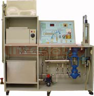
TEMPERATURE CONTROL LOOP TRAINER MODEL IBL-1
Temperature Control Loop Trainer Model TCL-1 is intended to study, how temperature in a heat exchanger can be controlled. Heat lost by a hot body is equal to heat gained by a cold body. This principle is used in this trainer. This instrument is used in instrumentation, electronics, and chemical engineering laboratories. In process industries, heat is transferred by radiation, by the mixing of hot and cold fluids, or, most frequently, by conduction through the walls of heat exchanger. A shell-and-tube heat exchanger is used in this instrument. The characteristic feature of this device is that the capacities on one or both sides are distributed along the length of the exchanger. The exit temperature of one fluid can be controlled by changing the temperature of the other fluid along the surface of the inner tubes. This is achieved by changing the rate of flow of cold-water inlet, so that the outlet temperature of the hot water is under control. There are several other considerations for control, but they are beyond the scope of this trainer. The heart of this trainer is a heat exchanger. This heat exchanger uses water as medium of transporting heat from hot water to cold water. Water is selected as a media, because water has finite specific constants (sp.gr = 1, boiling point @ 100? C, freezing point @ 0? C, 1cc weighs 1gm), and cannot be compressed like air. For these reasons, water provides stable operating conditions. Controlling hot water outlet temperature or cold water outlet temperature is accomplished in this instrument. The hot water in this heat exchanger flows through 14 numbers of seamless pipes, which are arranged in parallel, and passes on to the other side. All these seamless tubes are enclosed in a concentric outer shell, through which cold water flows. The construction is such that hot water and cold water do not come in contact. Heat is transmitted from hot water to cold water, by conduction, through these pipes. It is possible to measure the inlet and outlet of these hot and cold water. The controller can be activated to change the flow rate of cold water, by measuring hot water outlet temperature. The change in flow rate of cold water changes the outlet temperature of either cold water outlet or hot water outlet.
The Trainer contains:
Hot water boiler, to heat cold water coming from an over head tank (40Lt) placed above the instrument. Control valve to change the flow rate of cold water, by controlling I-P converter centrifugal pump to pump cold water from a built-in 60Lt sump. Rotometer to observe the flow rate of cold water, Four thermocouples measures hot and cold-water temperatures at inlet and outlet ports. A meter indicates the temperature on a panel meter by switch selection, Two solid state relays are used to switch ON 6 KW heaters. The hot water bath has necessary electronics to detect presence of water upto a minimum level before switching ON is provided as a protection measure. to an ON-OFF status of these heaters are indicated. Hand valves are placed at strategic points along the plumbing lines, All the above, assembled on a caster wheel based stand of 6' X 2' X 6'. Interface electronics, DC power supply, control software. IBM compatible computer. Dedicated interface card for the interface electronics, which occupies in one slot of the motherboard. Using this Trainer, we can perform the following experiments. 1.Execute program to scan inlet and outlet temperatures of cold water and hot water of the heat exchanger. Verify the same with the panel meter.
2. Run a program, to tabulate a relationship, between a digital to analog converter (DAC) and the 4-20mA current generated. This current can be monitored on digital indicator. Tabulate this relation DAC number (0-FF) Vs current output (4-20mA). Plot a graph
3. Study a program to change the stem position of control valve, under software control. The stem of the control valve changes its position from one extreme position to the other (usually 0 to 10-15mm) under air pressure. For 3PSI, the stem is in initial position, i.e., and 0mm. For 15PSI, the stem changes its position to the other end. This up/down movement causes, valve to open and close. This action changes the water flow through the pipeline. The water flow can be changed in the range of 3 to 10 Liters/min (LPM). This demonstrates how to change water flow pattern by software. Tabulate the input pressure (3-15 PSI) VS stem position (0 - 10mm). Plot a graph
4. Run PID control program for various bands. Many more experiments can be conducted in the above equipment, as every input and output element is accessible by software. You can formulate an experimental scheme to suit your syllabi needs. SOFTWARE:
In order to assist in conducting the experiment, several WINDOW based features are provided. They screens shown below are for setting the parameters and analysis.
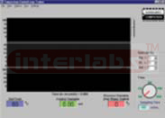
This is how the PID process screen looks like. It is necessary to enter the process parameters like Setpoint variable (SP), Proportional gain (Kp), Integral gain (Ki), Derivative gain (Kd), Sampling time in mS. This screen is displayed in response to the running of PID control program with the above parameter settings.
Upon saving this logged trend it is possible to make post analysis of the above controller. The following icons, represent various features available as post analysis options. Specifications: a) Control Valve:
Fluid : Water.
Body form : Globe-2-Way.
Size body/port/CV : 1/2"- 1/4" - 2.0 USGpm.
End Conn./Rating : Flanged RF - ANSI -150#.
Body material : CCS.
Trim form / Material : Contoured / SS304.
Flow chart/Direction : Linear / Under.
Actuator type : Diaphragm.
Control Signal : 0.2 - 1.0 Kg/cm2.
Valve action : Air to open.
Total stem travel : 18mm. b) Hand Operated Valves:
Quantity : 2 nos.
Size :1/2".
Coating : Nickel.
Type : Close open close. c) Gate Valve:
Quantity : 5Nos
Size : 1/2".
Service : Water. d) Heat Exchanger:
Construction : Shell-tube.
Service : Water.
Shell : 3".
Length : 30".
Tubes : 14 Nos. seam less.
Connections : 1/2" for inlet and outlet plumbing.
Drain : 4Nos gate valves. e) Electro-Pneumatic Converter:
Input : 4-20mA.
Output : 3-15 PSI.
Input Resistance : 90 Ohms.
Characteristics : Linear to input current.
Air supply :1.4Kg/cm2.
Consumption : 30 L/Hr typical.
Pressure : 1.4 bar.
Connection : 1/4" NPT.
Mounting :Wall. f) Air Filter Regulator:
Service media : Air.
Indicator : Pr gauges.
Max input : 10Kg/cm2.
Hose connection : 1/4" BSP. g) Solenoid:
Service : Water.
Coil Voltage : 220 VAC.
Service connection :1/2". h) Current Meters:
Digital : 0-20mA FSD. i) Rotometer:
Service : Water.
Connection : 1/2".
Range : 0 to 10.5 LPM.
Metering tube : Borosilicate.
Float : SS 304.
Needle : Provided, integral. j) Water Pump:
Voltage : 220V AC.
Lift : 2000 Lt./Hr at 20Meters high.
Service : Water.
Connection : 3/4" upstream.
1/2" reduced for downstream. k) Water Tank:
Sump : 1No.
Overhead : 1No.
Capacity : 100 Lt. Each.
Material : Toughened plastic. What you must provide the following facilities at your cost, at the time of installation:
You have to provide compressed air @ 5kg/cm2 from your in-house compressor.
Constant water line to be provided by you for filling the water tank and discharge pipelines must be provided to drain the water from the tank after the completion of the experiment.
You must provide an IBM Computer or Compatible system. It must have at least one vacant ISA slot on the motherboard, to enable the ADD-ON card to be inserted, which will communicate with the trainer. The minimum configuration of the system must be any Intel make standard CPU, 32MB RAM, one 1.44?FDD, HDD with any capacity, CD ROM drive, and a color monitor.
You must provide the necessary electrical fittings at 230V AC single phase, and accessories, observing all the safety standard features, like circuit breakers, safety switches and fuses etc, so that the operator will work under safe environment. Proper electrical grounding (earth) must be provided to the instrument setup as a whole.
This requires 10 Sq.ft floor space for conducting experiments by the students or trainee.
Good electrical connection, with proper earthing is required.
Mobility: Mounted on robust caster wheels
Dimensions : 6' X 2' X 6' (L, B, H)
Specifications are subject to change without notice. Changes in specifications may be effected even after receiving confirmed purchase ORDER.
See Enlarge
|
|
|
|
 Click to Enlarge
|
TEMPERATURE CONTROL LOOP TRAINER MODEL IBL-1
Temperature Control Loop Trainer Model TCL-1 is intended to study, how temperature in a heat exchanger can be controlled. Heat lost by a hot body is equal to heat gained by a cold body. This principle is used in this trainer. This instrument is used in instrumentation, electronics, and chemical engineering laboratories. In process industries, heat is transferred by radiation, by the mixing of hot and cold fluids, or, most frequently, by conduction through the walls of heat exchanger. A shell-and-tube heat exchanger is used in this instrument. The characteristic feature of this device is that the capacities on one or both sides are distributed along the length of the exchanger. The exit temperature of one fluid can be controlled by changing the temperature of the other fluid along the surface of the inner tubes. This is achieved by changing the rate of flow of cold-water inlet, so that the outlet temperature of the hot water is under control. There are several other considerations for control, but they are beyond the scope of this trainer. The heart of this trainer is a heat exchanger. This heat exchanger uses water as medium of transporting heat from hot water to cold water. Water is selected as a media, because water has finite specific constants (sp.gr = 1, boiling point @ 100? C, freezing point @ 0? C, 1cc weighs 1gm), and cannot be compressed like air. For these reasons, water provides stable operating conditions. Controlling hot water outlet temperature or cold water outlet temperature is accomplished in this instrument. The hot water in this heat exchanger flows through 14 numbers of seamless pipes, which are arranged in parallel, and passes on to the other side. All these seamless tubes are enclosed in a concentric outer shell, through which cold water flows. The construction is such that hot water and cold water do not come in contact. Heat is transmitted from hot water to cold water, by conduction, through these pipes. It is possible to measure the inlet and outlet of these hot and cold water. The controller can be activated to change the flow rate of cold water, by measuring hot water outlet temperature. The change in flow rate of cold water changes the outlet temperature of either cold water outlet or hot water outlet.
The Trainer contains:
Hot water boiler, to heat cold water coming from an over head tank (40Lt) placed above the instrument. Control valve to change the flow rate of cold water, by controlling I-P converter centrifugal pump to pump cold water from a built-in 60Lt sump. Rotometer to observe the flow rate of cold water, Four thermocouples measures hot and cold-water temperatures at inlet and outlet ports. A meter indicates the temperature on a panel meter by switch selection, Two solid state relays are used to switch ON 6 KW heaters. The hot water bath has necessary electronics to detect presence of water upto a minimum level before switching ON is provided as a protection measure. to an ON-OFF status of these heaters are indicated. Hand valves are placed at strategic points along the plumbing lines, All the above, assembled on a caster wheel based stand of 6' X 2' X 6'. Interface electronics, DC power supply, control software. IBM compatible computer. Dedicated interface card for the interface electronics, which occupies in one slot of the motherboard. Using this Trainer, we can perform the following experiments. 1.Execute program to scan inlet and outlet temperatures of cold water and hot water of the heat exchanger. Verify the same with the panel meter.
2. Run a program, to tabulate a relationship, between a digital to analog converter (DAC) and the 4-20mA current generated. This current can be monitored on digital indicator. Tabulate this relation DAC number (0-FF) Vs current output (4-20mA). Plot a graph
3. Study a program to change the stem position of control valve, under software control. The stem of the control valve changes its position from one extreme position to the other (usually 0 to 10-15mm) under air pressure. For 3PSI, the stem is in initial position, i.e., and 0mm. For 15PSI, the stem changes its position to the other end. This up/down movement causes, valve to open and close. This action changes the water flow through the pipeline. The water flow can be changed in the range of 3 to 10 Liters/min (LPM). This demonstrates how to change water flow pattern by software. Tabulate the input pressure (3-15 PSI) VS stem position (0 - 10mm). Plot a graph
4. Run PID control program for various bands. Many more experiments can be conducted in the above equipment, as every input and output element is accessible by software. You can formulate an experimental scheme to suit your syllabi needs. SOFTWARE:
In order to assist in conducting the experiment, several WINDOW based features are provided. They screens shown below are for setting the parameters and analysis.
This is how the PID process screen looks like. It is necessary to enter the process parameters like Setpoint variable (SP), Proportional gain (Kp), Integral gain (Ki), Derivative gain (Kd), Sampling time in mS. This screen is displayed in response to the running of PID control program with the above parameter settings.
Upon saving this logged trend it is possible to make post analysis of the above controller. The following icons, represent various features available as post analysis options. Specifications: a) Control Valve:
Fluid : Water.
Body form : Globe-2-Way.
Size body/port/CV : 1/2"- 1/4" - 2.0 USGpm.
End Conn./Rating : Flanged RF - ANSI -150#.
Body material : CCS.
Trim form / Material : Contoured / SS304.
Flow chart/Direction : Linear / Under.
Actuator type : Diaphragm.
Control Signal : 0.2 - 1.0 Kg/cm2.
Valve action : Air to open.
Total stem travel : 18mm. b) Hand Operated Valves:
Quantity : 2 nos.
Size :1/2".
Coating : Nickel.
Type : Close open close. c) Gate Valve:
Quantity : 5Nos
Size : 1/2".
Service : Water. d) Heat Exchanger:
Construction : Shell-tube.
Service : Water.
Shell : 3".
Length : 30".
Tubes : 14 Nos. seam less.
Connections : 1/2" for inlet and outlet plumbing.
Drain : 4Nos gate valves. e) Electro-Pneumatic Converter:
Input : 4-20mA.
Output : 3-15 PSI.
Input Resistance : 90 Ohms.
Characteristics : Linear to input current.
Air supply :1.4Kg/cm2.
Consumption : 30 L/Hr typical.
Pressure : 1.4 bar.
Connection : 1/4" NPT.
Mounting :Wall. f) Air Filter Regulator:
Service media : Air.
Indicator : Pr gauges.
Max input : 10Kg/cm2.
Hose connection : 1/4" BSP. g) Solenoid:
Service : Water.
Coil Voltage : 220 VAC.
Service connection :1/2". h) Current Meters:
Digital : 0-20mA FSD. i) Rotometer:
Service : Water.
Connection : 1/2".
Range : 0 to 10.5 LPM.
Metering tube : Borosilicate.
Float : SS 304.
Needle : Provided, integral. j) Water Pump:
Voltage : 220V AC.
Lift : 2000 Lt./Hr at 20Meters high.
Service : Water.
Connection : 3/4" upstream.
1/2" reduced for downstream. k) Water Tank:
Sump : 1No.
Overhead : 1No.
Capacity : 100 Lt. Each.
Material : Toughened plastic. What you must provide the following facilities at your cost, at the time of installation:
You have to provide compressed air @ 5kg/cm2 from your in-house compressor.
Constant water line to be provided by you for filling the water tank and discharge pipelines must be provided to drain the water from the tank after the completion of the experiment.
You must provide an IBM Computer or Compatible system. It must have at least one vacant ISA slot on the motherboard, to enable the ADD-ON card to be inserted, which will communicate with the trainer. The minimum configuration of the system must be any Intel make standard CPU, 32MB RAM, one 1.44?FDD, HDD with any capacity, CD ROM drive, and a color monitor.
You must provide the necessary electrical fittings at 230V AC single phase, and accessories, observing all the safety standard features, like circuit breakers, safety switches and fuses etc, so that the operator will work under safe environment. Proper electrical grounding (earth) must be provided to the instrument setup as a whole.
This requires 10 Sq.ft floor space for conducting experiments by the students or trainee.
Good electrical connection, with proper earthing is required.
Mobility: Mounted on robust caster wheels
Dimensions : 6' X 2' X 6' (L, B, H)
Specifications are subject to change without notice. Changes in specifications may be effected even after receiving confirmed purchase ORDER.
See Enlarge
|
|
|
|
 Click to Enlarge
|
FIELDBUS TRAINING SYSTEM
Foundation Fieldbus has developed standards that will enable process instrument manufacturers to mix and match, products manufactured by various manufacturers, while retaining their 4-20mA analog systems as it is. In short interoperability between various manufacturers is what is all about when they are connected in a network. This enables the operators to acquire field data from various plant control instruments and prepare archival, process trends, optimisation, and prepare health reports etc. This is because the field control instruments are made more intelligent by local microprocessors and pass, on-line data and messages to Fieldbus network. Thus it provides inputs for faster decision making. Fieldbus uses existing wiring and multi-drop connections, makes life lot easier when they are networked. Foundation Fieldbus training kit provides insight into this new generation instrumentation.
Foundation Fieldbus training kit is intended to study experiment and understand the concepts used in Foundation Fieldbus (FBUS) standards, while developing Foundation Fieldbus systems. The training kit consists of power supply, necessary components, cabling, connectors and devices. Useful for Instrumentation and control engineering students, electronics and communication engineers, plant operating trainees, system developers, and computer engineers.
Specifications:
Field bus HOST KIT Fieldbus Device Kit
Hardware Hardware
Fieldbus host kit 2 HI Fieldbus Round cards
ISA or PC Card interface board 2 AT-FBUS (ISA) interface boards
Optional device simulator Software
Software Communications stack
NI-FBUS Communications manager NI-FBUS Function block shell
NI-FBUS Configurator NI-FBUS Configurator
Lookout software with a Foundation Field bus driver NI-FBUS Monitor
Power supply and cabling. Power Supply and cabling.
Detailed information and specifications for the above products can be sent on request.
See Enlarge
|
|
|
|
|